
You are currently browsing the category archive for the ‘Theory of Numbers’ category.
Why primality is polynomial time, but factorisation is not
Differentiating between the signature of a number and its value
A brief review: The significance of evidence-based reasoning
In a paper: `The truth assignments that differentiate human reasoning from mechanistic reasoning: The evidence-based argument for Lucas’ Gödelian thesis’, which appeared in the December 2016 issue of Cognitive Systems Research [An16], I briefly addressed the philosophical challenge that arises when an intelligence—whether human or mechanistic—accepts arithmetical propositions as true under an interpretation—either axiomatically or on the basis of subjective self-evidence—without any specified methodology for objectively evidencing such acceptance in the sense of Chetan Murthy and Martin Löb:
“It is by now folklore … that one can view the values of a simple functional language as specifying evidence for propositions in a constructive logic …” … Chetan. R. Murthy: [Mu91], \S 1 Introduction.
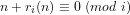
“Intuitively we require that for each event-describing sentence, 


Definition 1 (Evidence-based reasoning in Arithmetic): Evidence-based reasoning accepts arithmetical propositions as true under an interpretation if, and only if, there is some specified methodology for objectively evidencing such acceptance.
The significance of introducing evidence-based reasoning for assigning truth values to the formulas of a first-order Peano Arithmetic, such as PA, under a well-defined interpretation (see Section 3 in [An16]), is that it admits the distinction:
(1) algorithmically verifiable `truth’ (Definition 2}); and
(2) algorithmically computable `truth’ (Definition 3).
Definition 2 (Deterministic algorithm): A deterministic algorithm computes a mathematical function which has a unique value for any input in its domain, and the algorithm is a process that produces this particular value as output.
Note that a deterministic algorithm can be suitably defined as a `realizer‘ in the sense of the Brouwer-Heyting-Kolmogorov rules (see [Ba16], p.5).
For instance, under evidence-based reasoning the formula ![[(\forall x)F(x)]](https://s0.wp.com/latex.php?latex=%5B%28%5Cforall+x%29F%28x%29%5D+&bg=ffffff&fg=000000&s=-2&c=20201002)
![[F(x)]](https://s0.wp.com/latex.php?latex=%5BF%28x%29%5D+&bg=ffffff&fg=000000&s=-2&c=20201002)


Definition 2 (Algorithmic verifiability): The number-theoretical relation 


Whereas
Definition 3 (Algorithmic computability): The number theoretical relation 
The significance of the distinction between algorithmically computable reasoning based on algorithmically computable truth, and algorithmically verifiable reasoning based on algorithmically verifiable truth, is that it admits the following, hitherto unsuspected, consequences:
(i) PA has two well-defined interpretations over the domain 
(a) the weak non-finitary standard interpretation 
and
(b) a strong finitary interpretation 
(ii) PA is non-finitarily consistent under
(iii) PA is finitarily consistent under
The significance of evidence-based reasoning for Computational Complexity
In this investigation I now show the relevance of evidence-based reasoning, and of distinguishing between algorithmically verifiable and algorithmically computable number-theoretic functions (as defined above), for Computational Complexity is that it assures us a formal foundation for placing in perspective, and complementing, an uncomfortably counter-intuitive entailment in number theory—Theorem 2 below—which has been treated by conventional wisdom as sufficient for concluding that the prime divisors of an integer cannot be proven to be mutually independent.
However, I show there that such informally perceived barriers are, in this instance, illusory; and that admitting the above distinction illustrates:
(a) Why the prime divisors of an integer are mutually independent Theorem 2;
(b) Why determining whether the signature (Definition 3 below) of a given integer 


(c) Why it can be cogently argued that determining a factor of a given integer cannot be polynomial time.
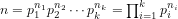
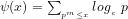
Definition 4 (Signature of a number): The signature of a given integer 

Unique since, if 


Definition 5 (Value of a number): The value of a given integer ![[n]](https://s0.wp.com/latex.php?latex=%5Bn%5D+&bg=ffffff&fg=000000&s=-2&c=20201002)
We note that Theorem 2 establishes a lower limit for [AKS04] and [LP11], because determining the signature of a given integer
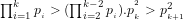
Theorem 1: (Fundamental Theorem of Arithmetic): Every positive integer 
where 

Are the prime divisors of an integer mutually independent?
In this paper I address the query:
Query 1: Are the prime divisors of an integer
Definition 6 (Independent events): Two events are independent if the occurrence of one event does not influence (and is not influenced by) the occurrence of the other.
Intuitively, the prime divisors of an integer seem to be mutually independent by virtue of the Fundamental Theorem of Arithmetic
Moreover, the prime divisors of 

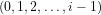
1, 2, 3, 4, 5, 6, 7, 8, 9, 10, 11, 12, 13, 14, 15, 16, 17, 18, 19 …
Despite such compelling evidence, conventional wisdom appears to accept as definitive the counter-intuitive conclusion that although we can see it as true, we cannot mathematically prove the following proposition as true:
Proposition 1: Whether or not a prime
We note that such an unprovable-but-intuitively-true conclusion makes a stronger assumption than that in Gödel’s similar claim for his arithmetical formula ![[(\forall x)R(x)]](https://s0.wp.com/latex.php?latex=%5B%28%5Cforall+x%29R%28x%29%5D+&bg=ffffff&fg=000000&s=-2&c=20201002)


![[R(n)]](https://s0.wp.com/latex.php?latex=%5BR%28n%29%5D+&bg=ffffff&fg=000000&s=-2&c=20201002)

Expressed in computational terms (see [An16], Corollary 8.3), under any well-defined interpretation of ![[R(x)]](https://s0.wp.com/latex.php?latex=%5BR%28x%29%5D+&bg=ffffff&fg=000000&s=-2&c=20201002)


![[\neg (\forall x)R(x)]](https://s0.wp.com/latex.php?latex=%5B%5Cneg+%28%5Cforall+x%29R%28x%29%5D+&bg=ffffff&fg=000000&s=-2&c=20201002)
We thus argue that a perspective which denies Proposition 1 is based on perceived barriers that reflect, and are peculiar to, only the argument that:
Theorem 2: There is no deterministic algorithm that, for any given 


Proof By a standard result in the Theory of Numbers ([Ste02], Chapter 2, p.9, Theorem 2.1, we cannot define a probability function for the probability that a random 
(Compare with the informal argument in [HL23], pp.36-37.)
In other words, treating Theorem 2 as an absolute barrier does not admit the possibility—which has consequences for the resolution of outstanding problems in both the theory of numbers and computational complexity—that Proposition 1 is algorithmically verifiable, but not algorithmically computable, as true, since:
Theorem 3: For any given
Author’s working archives & abstracts of investigations
![]()
(Notations, non-standard concepts, and definitions used commonly in these investigations are detailed in this post.)
A: A conventional perspective on why the prime divisors of an integer are not mutually independent
In a post Getting to the Roots of Factoring on the blog Gödel’s Lost Letter and P = NP (hosted jointly by him and Professor of Computer Science at Georgia Tech College of Computing, Richard Lipton) Professor of Computer Science and Engineering at the University of Buffalo, Kenneth W. Regan `revisits’ a 1994 paper on factoring by his co-host.
What I find intriguing in the above post is that the following extract subsumes, almost incidentally, a possibly implicit belief which may be inhibiting not only a resolution of the computational complexity of Integer Factoring (see this investigation) by conventional methods but, for similar reasons, also resolution of a large class of apparently unrelated problems (see, for instance, this investigation and this previous post):
“Here is the code of the algorithm. … the input 


Exiting enables carrying out the two prime factors of
How many iterations must one expect to make through this maze before exit? How and when can the choice of the polynomial
Note that we cannot consider the events 


The following reasoning shows why it is not obvious whether the assertion that:
“… we cannot consider the events
is intended to narrowly reflect a putative proof in the particular context of the assertion, or to echo a more general belief.
B: Defining the probability that a given integer is divisible by a given smaller integer
(1) We consider the questions:
(a) What is the probability for any given 


(b) What is the compound probability for any given 


(c) What is the compound probability for any given


C: Why the prime divisors of an integer are mutually independent
(2) We note that:
(a) The answer to query (1a) above is that the probability the roll of an 

(b) The answer to query (1b) above is that the probability the simultaneous roll of one 


(3) We trivially conclude that:
The compound probability of determining
(4) We further conclude non-trivially that the answer to query (1c) above is given by:
(a) If 
(b) The assumption that
For instance, let 


(5) We thus conclude non-trivially that, if
(Notations, non-standard concepts, and definitions used commonly in these investigations are detailed in this post.)
A: The twin prime conjecture
In the post Notes on the Bombieri asymptotic sieve on his blog What’s new, 2006 Fields Medal awardee and Professor of Mathematics at UCLA, Terence Tao, writes and comments that:
“The twin prime conjecture, still unsolved, asserts that there are infinitely many primes 

as 


Because
One can give a heuristic justification of the asymptotic (1) (and hence the twin prime conjecture) via sieve theoretic methods. …
It may also be possible that the twin prime conjecture could be proven by non-analytic means, in a way that does not lead to significantly new estimates on the sum 

B: Why heuristic approaches to the twin prime conjecture may not suffice
1. What seems to prevent a non-heuristic determination of the limiting behaviour of prime counting functions is that the usual approximations of 


2. The degree of approximation for finite values of
3. Moreover, currently, conventional approaches to evaluating prime counting functions for finite
(i) either—explicitly (see here)—that whether or not a prime 
(ii) or—implicitly (since the twin-prime problem is yet open)—that a proof to the contrary must imply that if 
4. If so, then conventional approaches seem to conflate the two probabilities:
(i) The probability 

Example 1: I have a bag containing 
(ii) The probability 
Example 2: I give you a 


5. In case 4(i), if the precise proportion of primes to non-primes in
However if 

6. In case 4(ii) it follows that 
7. We thus have that 

8. Moreover, by considering the asymptotic density of the set of all integers that are not divisible by the first 


9. We can then show that a non-heuristic approximation for the number of primes less than or equal to

for some constant 
10. We can show, similarly, that the expected number of Dirichlet and twin primes in the interval (


11. The method can, moreover, be generalised to apply to a large class of prime counting functions (see Section 5.A on p.22 of this investigation).
C: A non-heuristic proof that there are infinitely many twin primes
1. In particular, instead of estimating:
heuristically by analytic considerations, one could also estimate the number 


where 
2. One way of approaching this would be to define an integer 


3. Note that if 


4. The asymptotic density of
5. Further, if 

6. If we define 


7. Since 


8. Now, the expected number of

9. We conclude that the number 


Author’s working archives & abstracts of investigations
![]()
(Notations, non-standard concepts, and definitions used commonly in these investigations are detailed in this post.)
We investigate whether the probabilistic distribution of prime numbers can be treated as a heuristic model of quantum behaviour, since it too can be treated as a quantum phenomena, with a well-defined binomial probability function that is algorithmically computable, where the conjectured values of 
1. Thesis: The concept of ‘mathematical truth’ must be accountable
The thesis of this investigation is that a major philosophical challenge—which has so far inhibited a deeper understanding of the quantum behaviour reflected in the mathematical representation of some laws of nature (see, for instance, this paper by Eamonn Healey)—lies in holding to account the uncritical acceptance of propositions of a mathematical language as true under an interpretation—either axiomatically or on the basis of subjective self-evidence—without any specified methodology of accountability for objectively evidencing such acceptance.
2. The concept of ‘set-theoretical truth’ is not accountable
Since current folk lore is that all scientific truths can be expressed adequately, and communicated unambiguously, in the first order Set Theory ZF, and since the Axiom of Infinity of ZF cannot—even in principle—be objectively evidenced as true under any putative interpretation of ZF (as we argue in this post), an undesirable consequence of such an uncritical acceptance is that the distinction between the truths of mathematical propositions under interpretation which can be objectively evidenced, and those which cannot, is not evident.
3. The significance of such accountability for mathematics
The significance of such a distinction for mathematics is highlighted in this paper due to appear in the December 2016 issue of Cognitive Systems Research, where we address this challenge by considering the two finitarily accountable concepts of algorithmic verifiability and algorithmic computability (first introduced in this paper at the Symposium on Computational Philosophy at the AISB/IACAP World Congress 2012-Alan Turing 2012, Birmingham, UK).
(i) Algorithmic verifiability
A number-theoretical relation 


(ii) Algorithmic computability
A number theoretical relation 

(iii) Algorithmic verifiability vis à vis algorithmic computability
We note that algorithmic computability implies the existence of an algorithm that can decide the truth/falsity of each proposition in a well-defined denumerable sequence of propositions, whereas algorithmic verifiability does not imply the existence of an algorithm that can decide the truth/falsity of each proposition in a well-defined denumerable sequence of propositions.
From the point of view of a finitary mathematical philosophy—which is the constraint within which an applied science ought to ideally operate—the significant difference between the two concepts could be expressed by saying that we may treat the decimal representation of a real number as corresponding to a physically measurable limit—and not only to a mathematically definable limit—if and only if such representation is definable by an algorithmically computable function (Thesis 1 on p.9 of this paper that was presented on 26th June at the workshop on Emergent Computational Logics at UNILOG’2015, 5th World Congress and School on Universal Logic, Istanbul, Turkey).
We note that although every algorithmically computable relation is algorithmically verifiable, the converse is not true.
We show in the CSR paper how such accountability helps define finitary truth assignments that differentiate human reasoning from mechanistic reasoning in arithmetic by identifying two, hitherto unsuspected, Tarskian interpretations of the first order Peano Arithmetic PA, under both of which the PA axioms interpret as finitarily true over the domain
4. The ambit of human reasoning vis à vis the ambit of mechanistic reasoning
One corresponds to the classical, non-finitary, putative standard interpretation of PA over
The other corresponds to a finitary interpretation of PA over
5. The significance of such accountability for the mathematical representation of physical phenomena
The significance of such a distinction for the mathematical representation of physical phenomena is highlighted in this paper that was presented on 26th June at the workshop on Emergent Computational Logics at UNILOG’2015, 5th World Congress and School on Universal Logic, Istanbul, Turkey, where we showed how some of the seemingly paradoxical elements of quantum mechanics may resolve if we define:
Quantum phenomena: A phenomena is a quantum phenomena if, and only if, it obeys laws that can only be represented mathematically by functions that are algorithmically verifiable but not algorithmically computable.
6. The mathematical representation of quantum phenomena that is determinate but not predictable
By considering the properties of Gödel’s 

However, since the algorithmic verifiability of any quantum phenomena shows that it is mathematically determinate, it follows that the physical phenomena itself must observe determinate laws.
7. Such representation does not need to admit multiverses
Hence (contrary to any interpretation that admits unverifiable multiverses) only one algorithmically computable extension of the function is consistent with the law determining the behaviour of the phenomena, and each possible extension must therefore be associated with a probability that the next observation of the phenomena is described by that particular extension.
8. Is the probability of the future behaviour of quantum phenomena definable by an algorithmically computable function?
The question arises: Although we cannot represent quantum phenomena explicitly by an algorithmically computable function, does the phenomena lend itself to an algorithmically computable probability of its future behaviour in the above sense?
9. Can primes yield a heuristic model of quantum behaviour?
We now show that the distribution of prime numbers denoted by the arithmetical prime counting function
10. Two prime probabilities
We consider the two probabilities:
(i) The probability
Example 1: I have a bag containing
(ii) The probability
Example 2: I give you a
11. The probability of a randomly chosen number from the set of natural numbers is not definable
Clearly the probability
However if 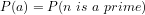
12. The prime divisors of a natural number are independent
Now, the following paper proves
Why Integer Factorising cannot be polynomial time
We thus have that
Hence, even though we cannot define the probability
13. The distribution of primes is a quantum phenomena
The distribution of primes is thus determinate but unpredictable, since it is representable by the algorithmically verifiable but not algorithmically computable arithmetical number-theoretic function 

The Prime Number Generating Theorem and the Trim and Compact algorithms detailed in this 1964 investigation illustrate why the arithmetical number-theoretic function 
Moreover, although the distribution of primes is a quantum phenomena with probabilty
14. Why the universe may be algorithmically computable
By analogy, this suggests that although the measurable values of some individual properties of particles in the universe over time may represent a quantum phenomena, the universe itself may be algorithmically computable if the laws governing the generation of all the particles in the universe over time are algorithmically computable.
Author’s working archives & abstracts of investigations
![]()
Notations, non-standard concepts, and definitions used commonly in these investigations are detailed in this post.)
1. Since, by the Prime Number Theorem, the number of primes 


2. Currently, conventional approaches to determining the computational complexity of Integer Factorising apparently appeal critically to the belief that:
(i) either—explicitly (see here)—that whether or not a prime
(ii) or—implicitly (since the problem is yet open)—that a proof to the contrary must imply that if
3. If so, then conventional approaches seem to conflate the two probabilities:
(i) The probability
Example 1: I have a bag containing
(ii) The probability
Example 2: I give you a
4. In case 3(i), if the precise proportion of primes to non-primes in
However if
5. In case 3(ii) the following paper proves
Why Integer Factorising cannot be polynomial time
Not only does it immediately follow that
Author’s working archives & abstracts of investigations
![]()

1 The Riemann Hypothesis (see also this paper) reflects the fact that all currently known approximations of the number
All known approximations of the number
The above graph compares the actual number 


1A Two non-heuristic approximations of the number
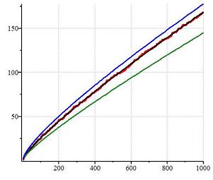
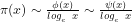
The following introduces, and compares, two non-heuristic prime counting functions (investigated more fully here) that, prima facie, yield non-heuristic approximations of
(i) 
(ii) 
Based on manual and spreadsheet calculations, Figs.1 and 2 compare the values of the two non-heuristically estimated prime counting functions with the actual values of 

Fig.1: The above graph compares the non-heuristically estimated values of 


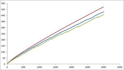
Fig.2: The above graph compares the non-heuristically estimated values of 


1B Three intriguing queries
Since 


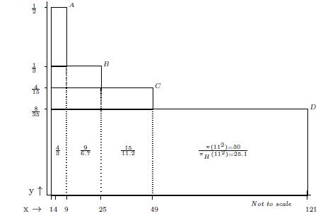
Fig.3. The overlapping rectangles 


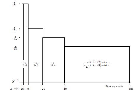
Fig.4: Graph of 
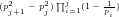


(a) Which is the least 
(b) Which is the largest 
(c) Is 

1C Three intriguing observations
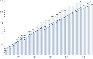
Fig.5: The above graph compares the actual values of 


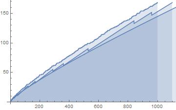
Fig.6: The above graph compares the actual values of 


Fig.7: The above graph compares the actual values of 


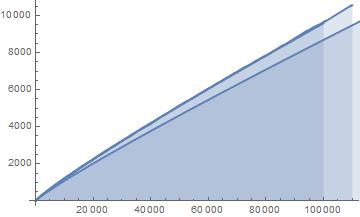
Fig.8: The above graph compares the actual values of 


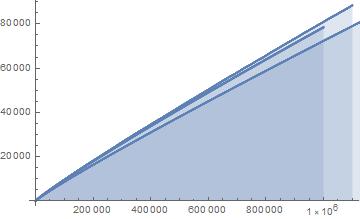
Fig.9: The above graph compares the actual values of 


Query (a) is answered by Figs.8-9, which show that the least 
As regards Query (b) however, we conjecture that Fig.9 suggests that there is no larger
Finally, we conjecture that—despite what is suggested by the Prime Number Theorem—Query (c) can be answered affirmatively if the three functions 

2 Density of integers not divisible by primes
The above observations reflect the circumstance that (formal proofs for the following are detailed in Chapters 34 and 35 here):
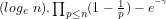
Lemma 2.1: The asymptotic density of the set of all integers that are not divisible by any of a given set of primes 

It follows that:
Lemma 2.2: The expected number of integers in any interval 
2A The function
In particular, the expected number 


Corollary 2.3:

It follows that:
Corollary 2.4: The expected number of primes 
We conclude that
Lemma 2.5: 
2B The function
We note similarly that:
Corollary 2.6: The expected number of primes in the interval (

It further follows from Lemma 2.2 and Corollary 2.6 that:
Corollary 2.7: The number 


We conclude that 
Lemma 2.8: 
2C An apparent paradox
We note that since the above non-heuristic estimates appeal to an asymptotic density, and the density of primes tends to 
(i) 
(ii)
even though Fig.3 suggests that:


In other words, an apparent paradox surfaces (as suggested by Fig.9) when we express 


Since 


We conclude that:
Theorem For any given 


Since 


Corollary The Prime Number Theorem implies that:

3 Conventional estimates of 

We note that Guy Robin (Robin, G. (1983). “Sur l’ordre maximum de la fonction somme des diviseurs”. Séminaire Delange-Pisot-Poitou, Théorie des nombres (1981-1982). Progress in Mathematics. 38: 233-244.) proved (implicit assumptions?) that the following changes sign infinitely often:
Robin’s result is analogous to Littlewood’s curious theorem (implicit assumptions?) that the difference 


Littlewood’s theorem is `curious’ since:
(a) There is no explicitly defined arithmetical formula that, for any 


(b) Littlewood’s proof deduces the behaviour of 
Moreover, we note that—unlike 

where:

and, as detailed here, the latter is curiously stipulated as valid only for 

“

for 

![]()
(Notations, non-standard concepts, and definitions used commonly in these investigations are detailed in this post.)


In a 2005 Clay Math Institute invited large lecture to a popular audience at MIT ‘Are there still unsolved problems about the numbers
“If I give you a number
Although this may represent conventional wisdom, it is not, however, strictly true!
Reason: The following 1964 Theorem yields two algorithms (Trim/Compact), each of which affirmatively answers the questions:
(i) Do we necessarily discover the primes in a Platonic domain of the natural numbers, as is suggested by the sieve of Eratosthenes, or can we also generate them sequentially in a finitarily definable domain that builds into them the property of primality?
(ii) In other words, given the first 

I: A PRIME NUMBER GENERATING THEOREM
Theorem: For all 


and:

Let 

Then:

Proof: For all
Since 

Hence:
and so it is the prime
II: TRIM NUMBERS
The significance of the Prime Number Generating Theorem is seen in the following algorithm.
We define Trim numbers recursively by 
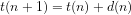
(1) 


(2) 
(3)


It follows that the Trim number 
The Trim Number Algorithm

n
1 2 2 3 5 7 11 13 17 19 23 27 29 31 37
2 3 1 
3 5 1 1
4 7 1 2 3 
5 11 1 1 4 3
6 13 1 2 2 1 9
7 17 1 1 3 4 5 9
8 19 1 2 1 2 3 7 15
9 23 1 1 2 5 10 3 11 15
10 27 1 0 3 1 6 12 7 11 19
11 29 1 1 1 6 4 10 5 9 17

n 


NOTE: The first 


(i) Trim composite 

(ii) Trim composite 

(iii) Trim composite 

(iv) Trim composite 

Theorem: For all

II A:
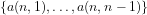
For any given natural number 


(1)
(2) 
(3)

It follows that the 

III: COMPACT NUMBERS
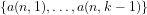
Compact numbers are defined recursively by 
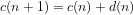
(1)
(2) 
(3)

(4)

(5) 

It follows that the compact number 

The Compact Number Algorithm
n
1 2 2 3 5 7 11 13 17 19 23 29 31 37 41
2 3 1
3 5 1
4 7 1
5 9 1 0
6 11 1 1
7 13 1 2
8 17 1 1
9 19 1 2
10 23 1 1
11 25 1 2 0
12 29 1 1 1
13 31 1 2 4 
14 37 1 2 3
15 41 1 1 4
16 43 1 2 2
17 47 1 1 3
18 49 1 2 1 0
19 53 1 1 2 3
20 57 1 0 3 6
21 59 1 1 1 4
22 61 1 2 4 2
23 67 1 2 3 3
24 71 1 1 4 6
25 73 1 2 2 4
26 79 1 2 1 5
27 83 1 1 2 1
28 87 1 0 3 4
29 89 1 1 1 2
30 93 1 0 2 5
31 97 1 2 3 1
32 101 1 1 4 4
33 103 1 2 2 2
34 107 1 1 3 5
35 109 1 2 1 3
36 113 1 1 2 6
37 117 1 0 3 2
38 121 1 2 4 5 0
39 127 1 2 3 6 5
40 131 1 1 4 2 1
41 137 1 1 3 3 6
42 139 1 2 1 1 4
43 145 1 2 0 2 9
44 149 1 1 1 5 5
45 151 1 2 4 5 0
46 157 1 2 3 4 8
47 163 1 2 2 5 2
48 167 1 1 3 1 9
49 169 1 2 1 6 7 0
50 173 1 1 2 2 3 9
51 177 1 0 3 5 10 5
52 179 1 1 1 3 8 3
53 181 1 2 4 1 6 1 
54 189 1 0 1 0 9 6
55 191 1 1 4 5 7 4
56 193 1 2 2 3 5 2
57 197 1 1 3 6 1 11
58 199 1 2 1 4 10 9
59 205 1 2 0 5 4 3
60 211 1 2 4 6 9 10
61 219 1 0 1 5 1 2
62 223 1 2 2 1 8 11
63 227 1 1 3 4 4 7
64 229 1 2 1 2 2 5
65 233 1 1 2 5 9 14
66 237 1 0 3 1 5 10
67 239 1 1 1 6 3 8
68 241 1 2 4 4 1 6
69 249 1 0 1 3 4 11
70 251 1 1 4 1 2 9
71 257 1 1 3 2 7 3
72 261 1 0 4 5 3 12
73 263 1 1 2 3 1 10
74 267 1 0 3 6 8 6
75 269 1 1 1 4 6 4
76 271 1 2 4 2 4 2
77 277 1 2 3 3 9 9
78 281 1 1 4 6 5 5
79 283 1 2 2 4 3 3
n 
NOTE: The first 


Theorem 1: There is always a Compact Number 

Theorem 2: For sufficiently large 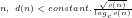

A later investigation (see also this post) shows why the usual, linearly displayed, Eratosthenes sieve argument reveals the structure of divisibility (and, ipso facto, of primality) more transparently when displayed as the 1964, 


‘Density‘: For instance, the residues 


Fig.1
Sequence 


n=1 
n=2 0
n=3 0 1
n=4 0 0 2
n=5 0 1 1 3
n=6 0 0 0 2 4
n=7 0 1 2 1 3 5
n=8 0 0 1 0 2 4 6
n=9 0 1 0 3 1 3 5 7
n=10 0 0 2 2 0 2 4 6 8
n=11 0 1 1 1 4 1 3 5 7 9
n
We note that:


Primality: The residues 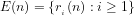
Fig.2
Sequence


We note that:


The significance of expressing Eratosthenes sieve as a
Fig.1 illustrates that although the probability
The probability
Fig.2 illustrates, however, that the probability 
We thus have that
The putative non-heuristic probability that a given
Hence, even though we cannot define the probability

The significance of the above perspective is that (see this investigation) it admits non-heuristic approximations of prime counting functions (see Fig.15 of the investigation) where:
“It has long been known that that for any real number 


… Barry Mazur and William Stein, ‘What is Riemann’s Hypothesis‘
![]()
This argument laid the foundation for this investigation. See also this arXiv preprint, and this broader update.
Abstract We define the residues 


We begin by defining the residues
Definition 1:
Since each residue 

It immediately follows that:
Lemma 1: 
By the standard definition of the probability 

Lemma 2: For any 


We note the standard definition:
Definition 2: Two events 

We then have that:
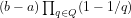
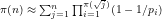
Lemma 3: If 


where 

Proof: The 


By Lemma 2:

The lemma follows.

If 

Corollary 1: 
Corollary 2: 
Theorem 1: The prime divisors of any integer

Since 
Lemma 4: For any 

Lemma 5: 

The number of primes less than or equal to
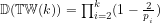
Lemma 6: 
This now yields the Prime Number Theorem:
Theorem 2: 
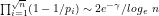
Proof: From Lemma 6 and Mertens’ Theorem that
[5]:

it follows that:


![(\pi(x).log_{e}\ x)/x \sim c.(log_{e}\ x/x)[log_{e}.log_{e}\ t + log_{e}\ t + \sum_{2}^{\infty}(log_{e}\ t)^{k}/(k. k!)]_{2}^{^{x}}](https://s0.wp.com/latex.php?latex=%28%5Cpi%28x%29.log_%7Be%7D%5C+x%29%2Fx+%5Csim+c.%28log_%7Be%7D%5C+x%2Fx%29%5Blog_%7Be%7D.log_%7Be%7D%5C+t+%2B+log_%7Be%7D%5C+t+%2B+%5Csum_%7B2%7D%5E%7B%5Cinfty%7D%28log_%7Be%7D%5C+t%29%5E%7Bk%7D%2F%28k.+k%21%29%5D_%7B2%7D%5E%7B%5E%7Bx%7D%7D&bg=ffffff&fg=000000&s=-2&c=20201002)
![(\pi(x).log_{e}\ x)/x \sim c.(log_{e}\ x/x)[log_{e}.log_{e}\ x + log_{e}\ x + \sum_{2}^{\infty}(log_{e}\ x)^{k}/(k. k!)]](https://s0.wp.com/latex.php?latex=%28%5Cpi%28x%29.log_%7Be%7D%5C+x%29%2Fx+%5Csim+c.%28log_%7Be%7D%5C+x%2Fx%29%5Blog_%7Be%7D.log_%7Be%7D%5C+x+%2B+log_%7Be%7D%5C+x+%2B+%5Csum_%7B2%7D%5E%7B%5Cinfty%7D%28log_%7Be%7D%5C+x%29%5E%7Bk%7D%2F%28k.+k%21%29%5D&bg=ffffff&fg=000000&s=-2&c=20201002)

The behaviour of 


Hence
Acknowledgements
I am indebted to my erstwhile classmate, Professor Chetan Mehta, for his unqualified encouragement and support for my scholarly pursuits over the past fifty years; most pertinently for his patiently critical insight into the required rigour without which the argument of this 1964 investigation would have remained in the informal universe of seemingly self-evident truths.
References
HW60 G. H. Hardy and E. M. Wright. 1960. An Introduction to the Theory of Numbers 4th edition. Clarendon Press, Oxford.
Ti51 E. C. Titchmarsh. 1951. The Theory of the Riemann Zeta-Function. Clarendon Press, Oxford.
Notes
Return to 1: HW60, p.49.
Return to 2: HW60, p.52, Theorem 59.
Return to 3: In the previous post we have shown how it immediately follows from Theorem 1 that integer factorising is necessarily of order 

Return to 4: By HW60, p.351, Theorem 429, Mertens’ Theorem.
Return to 5: By the argument in Ti51, p.59, eqn.(3.15.2).
Return to 6: HW60, p.9, Theorem 7.
Author’s working archives & abstracts of investigations
![]()
This argument laid the foundation for this later post and this investigation.
(Notations, non-standard concepts, and definitions used commonly in these investigations are detailed in this post.)
Abstract: We show the joint probability 
We define the residues
Definition 1:
Since each residue
We note that:
Lemma 1:
By the standard definition of the probability [2]
Lemma 2: For any
We note the standard definition [3]:
Definition 2: Two events
We then have that:
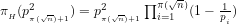
Lemma 3: If
where
Proof: The
By Lemma 2:
The lemma follows.
If
Corollary 1:
Corollary 2:
Theorem 1: The prime divisors of any integer
Since
It then immediately follows from Theorem 1 that:
Corollary 3: Integer Factorising is not in
Proof: We note that any computational process to identify a prime divisor of
Since
Moreover, since the number of such primes is of the order 

The corollary follows if
Acknowledgements
I am indebted to my erstwhile classmate, Professor Chetan Mehta, for his unqualified encouragement and support for my scholarly pursuits over the past fifty years; most pertinently for his patiently critical insight into the required rigour without which the argument of this 1964 investigation would have remained in the informal universe of seemingly self-evident truths.
References
GS97 Charles M. Grinstead and J. Laurie Snell. 1997. Introduction to Probability. Second Revised Edition, 1997, American Mathematical Society, Rhode Island, USA.
HW60 G. H. Hardy and E. M. Wright. 1960. An Introduction to the Theory of Numbers 4th edition. Clarendon Press, Oxford.
Ko56 A. N. Kolmogorov. 1933. Foundations of the Theory of Probability. Second English Edition. Translation edited by Nathan Morrison. 1956. Chelsea Publishing Company, New Yourk.
An05 Bhupinder Singh Anand. 2005. Three Theorems on Modular Sieves that suggest the Prime Difference is 
Notes
Return to 1: HW60, p.49.
Return to 2: Ko56, Chapter I, Section 1, Axiom III, p.2; see also GS97, Chapter 1, Section 1.2, Definition 1.2, p.19.
Return to 3: Ko56, Chapter VI, Section 1, Definition 1, pg.57 and Section 2, pg.58; see also GS97, Chapter 4, Section 4.1, Theorem 4.1, pg.140.
Return to 4: HW60, p.52, Theorem 59.
Author’s working archives & abstracts of investigations
![]()
In this post we shall beg indulgence for wilfully ignoring Wittgenstein’s dictum: “Whereof one cannot speak, thereof one must be silent.”
(Notations, non-standard concepts, and definitions used commonly in these investigations are detailed in this post.)

In his comments on this earlier post (on the need for a better consensus on the definition of `effective computability‘) socio-proctologist Vivek Iyer—who apparently prefers to be known here only through this blogpage, and whose sustained interest has almost compelled a more responsible response in the form of this blogpage—raised an interesting query (albeit obliquely) on whether commonly accepted Social Welfare Functions—such as those based on Muth rationality—could possibly be algorithmically verifiable, but not algorithmically computable:
“We know the mathematical properties of market solutions but assume we can know the Social Welfare Function which brought it about. We have the instantiation and know it is computable but we don’t know the underlying function.”
He later situated the query against the perspective of:
“… the work of Robert Axtell http://scholar.google.com/citations?user=K822uYQAAAAJ&hl=en- who has derived results for the computational complexity class of market (Walrasian) eqbm. This is deterministically computable as a solution for fixed points in exponential time, though easily or instantaneously verifiable (we just check that the market clears by seeing if there is anyone who still wants to sell or buy at the given price). Axtell shows that bilateral trades are complexity class P and this is true of the Subjective probabilities.”
Now, the key para of Robert Axtell’s paper seemed to be:
“The second welfare theorem states that any Pareto optimal allocation is a Walrasian equilibrium from some endowments, and is usually taken to mean that a social planner/society can select the allocation it wishes to achieve and then use tax and related regulatory policy to alter endowments such that subsequent market processes achieve the allocation in question. We have demonstrated above that the job of such a social planner would be very hard indeed, and here we ask whether there might exist a computationally more credible version of the second welfare theorem”…Axtell p.9
Axtell’s aim here seemed to be to maximise in polynomial time the Lyapunov function 
Prima facie Axtell’s problem seemed to lie within a general class of problems concerning the distribution of finite resources amongst a finite population.
For instance, the total number of ways, say 


We noted that if we take one of the allocations 
We assumed there that, for any given set of distributions 


We noted that mathematically the above can be viewed as a variation of the Travelling Salesman problem where the goal is to minimise the total cost of progressing from a starting distribution 
We further noted that, since the Travelling Salesman Problem is in the complexity class 


In order to get a better perspective on the issue of an equilibrium, we shall now speculate on whether we can reasonably define a market equilibrium in a simplified terminating market situation (i.e., a situation which always ends when there is no possible further profitable activity for any participant), where our definition of an equilibrium is any terminal state of minimum total cost and maximum total gain.
For instance, we could treat the population in question as a simplified on-line Stock Exchange with 

Now we can represent a distribution 


We note that the generating function for
One could then conceive of a Transaction Corpus Tax (


Now, given an initial distribution, say 


Obviously the gain to 
However, what is important to note here (which obviously need not apply in dissimilar cases such as Axtell’s) is that apparently none of the following factors:
(a) the price of the scrip being traded at any transaction;
(b) the quantum of the gain (which need not even be quantifiable in any particular transaction);
(c) the quantum of
seem to play any role in reaching the Equilibrium Distribution 

Moreover, the only restriction is on


In other words, no transaction can take place that requires a distribution to be repeated.
One way of justifying such a Regulatory restriction would be that if a distribution were allowed to repeat itself, a cabal could prevent market equilibrium by artificially fuelling speculation aimed at merely inflating the valuations of the
By definition, starting with any distribution 
If so, this would reduce the above to a Travelling Salesman Problem TSP if we define the Equilibrium Distribution
In other words, the Equilibrium Distribution is—by definition—the one for which 

Assuming all the speculators
In other words, in the worst case where the quantum of Transaction Corpus Tax can be arbitrarily revised and levied with retrospective effect at any transaction, is there a Nash strategy that can guide the set
References
Ax03 Robert Axtell. 2003. The Complexity of Exchange. In Econometrica, Vol. 29, No. 3 (July 1961).
Mu61 John F. Muth. 1961. Rational Expectations and the Theory of Price Movements. In Econometrica, Vol. 29, No. 3 (July 1961).
![]()

Recent comments